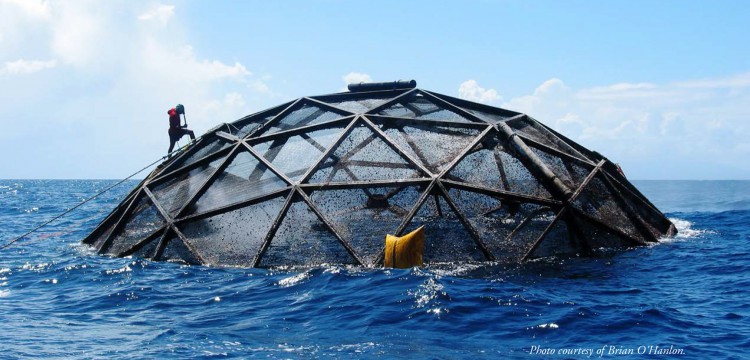
Prioritizing Potential Aquaculture Zones

NOAA Supports Development of Offshore Aquaculture in Southern California

Background

Marine aquaculture could become a key contributor to the world’s food supply, offering a more sustainable protein source than terrestrial meat production.¹ Gentry  et  al. mapped the global potential for marine aquaculture by considering constraints such as ship traffic, dissolved‑oxygen levels, and seabed depth. Their analysis showed that the projected demand for seafood could be satisfied using under 0.015 % of the planet’s ocean surface.² Additionally, aquaculture contributed $885.7 million (USD) to the U.S Western Region and supported more than 6,000 jobs in 2022.³ Shellfish alone, accounted for $360.6 million of this total amount. Placement of aquaculture farms along the coast for a particular species needs to be given special consideration. In the following analysis, bathymetry data and average sea surface temperature data will be combined to estimate the total amount of suitable aquaculture area for a species within West Coast Exclusive Economic Zones given their optimal depth and temperature ranges. Exclusive Economic Zones (EEZs) are areas in which the U.S. and other coastal nations have jurisdiction over natural resources.⁴

Data

Sea surface temperature (SST): raster data from the years 2008 to 2012 to characterize the average sea surface temperature within the region generated from NOAA’s 5km Daily Global Satellite Sea Surface Temperature Anomaly v3.1.⁵

Bathymetry data: raster data of ocean depth retrieved from General Bathymetric Chart of the Oceans (GEBCO).⁶

Exclusive Economic Zones (EEZs): shapefiles of West coast regions of US from Marineregions.org. These regions are Washington, Oregon, Northern California, Central California, and Southern California.⁷

Prepare data

Import necessary packages.

Code

library(tidyverse)
library(here)
library(dplyr)
library(sf)
library(terra)
library(stars)
library(tmap)
library(knitr)
library(kableExtra)
library(patchwork)

Load all necessary data.

Code

# Import Average Annual SST data from 2008-2012 

sst_2008 <- rast(here("blogposts", "prioritizing-aquaculture", "data", "average_annual_sst_2008.tif"))
sst_2009 <- rast(here("blogposts", "prioritizing-aquaculture", "data", "average_annual_sst_2009.tif"))
sst_2010 <- rast(here("blogposts", "prioritizing-aquaculture", "data", "average_annual_sst_2010.tif"))
sst_2011 <- rast(here("blogposts", "prioritizing-aquaculture", "data", "average_annual_sst_2011.tif"))
sst_2012 <- rast(here("blogposts", "prioritizing-aquaculture", "data", "average_annual_sst_2012.tif"))

# Import bathymetry data

depth <- rast(here("blogposts", "prioritizing-aquaculture", "data", "depth.tif"))

# Import exclusive economic zones off west coast 

regions <- st_read(here("blogposts", "prioritizing-aquaculture", "data", "wc_regions_clean.shp"))

Process data

Processing begins with the sea‑surface‑temperature (SST) raster data. When working with multiple geospatial layers, the first and most important step is to confirm that every dataset uses the same coordinate reference system (CRS). Even though the SST rasters come from the same source and are probably already aligned, the CRS of each layer should be explicitly checked to guarantee consistency before proceeding.

Code

cat(
  "CRS(sst_2008) == CRS(sst_2009):", crs(sst_2008) == crs(sst_2009), "\n",
  "CRS(sst_2009) == CRS(sst_2010):", crs(sst_2009) == crs(sst_2010), "\n",
  "CRS(sst_2010) == CRS(sst_2011):", crs(sst_2010) == crs(sst_2011), "\n",
  "CRS(sst_2011) == CRS(sst_2012):", crs(sst_2011) == crs(sst_2012), "\n")

CRS(sst_2008) == CRS(sst_2009): TRUE 
 CRS(sst_2009) == CRS(sst_2010): TRUE 
 CRS(sst_2010) == CRS(sst_2011): TRUE 
 CRS(sst_2011) == CRS(sst_2012): TRUE

Code

print(crs(sst_2008))

[1] "GEOGCRS[\"WGS 84\",\n    DATUM[\"unknown\",\n        ELLIPSOID[\"WGS84\",6378137,298.257223563,\n            LENGTHUNIT[\"metre\",1,\n                ID[\"EPSG\",9001]]]],\n    PRIMEM[\"Greenwich\",0,\n        ANGLEUNIT[\"degree\",0.0174532925199433,\n            ID[\"EPSG\",9122]]],\n    CS[ellipsoidal,2],\n        AXIS[\"latitude\",north,\n            ORDER[1],\n            ANGLEUNIT[\"degree\",0.0174532925199433,\n                ID[\"EPSG\",9122]]],\n        AXIS[\"longitude\",east,\n            ORDER[2],\n            ANGLEUNIT[\"degree\",0.0174532925199433,\n                ID[\"EPSG\",9122]]]]"

The output shows that each yearly SST raster shares the same CRS (EPSG 9122), confirming a consistent projection.

Next, the rasters for 2008–2012 are merged into a single stack, the per‑pixel mean across those years is calculated, and the resulting values are converted from Kelvin to Celsius by subtracting 273.15 °C. This produces a single raster representing the average sea‑surface temperature (°C) for the 2008–2012 period.

Code

# Create single raster stack of SST 

stacked_sst <- c(sst_2008, sst_2009, sst_2010, sst_2011, sst_2012)

# Find average and convert to Celsius  
avg_sst_c <- mean(stacked_sst) - 273.15

Now the SST, depth, and EEZ data need to be processed so they can be combined. All datasets must share the same CRS, extent, and resolution. A check will be run to determine what modifications are required before merging the datasets.

Code

# Checking if CRS, resolutions, and extents of all data match.

cat(
  "CRS(avg_sst_c) == CRS(depth):", crs(avg_sst_c) == crs(depth), "\n",
  "RES(avg_sst_c) == RES(depth):", res(avg_sst_c) == res(depth), "\n",
  "EXT(avg_sst_c) == EXT(depth):", ext(avg_sst_c) == ext(depth), "\n",
  "CRS(avg_sst_c) == CRS(regions):", crs(avg_sst_c) == crs(regions), "\n",
  "EXT(avg_sst_c) == EXT(regions):", ext(avg_sst_c) == ext(regions), "\n"
)

CRS(avg_sst_c) == CRS(depth): FALSE 
 RES(avg_sst_c) == RES(depth): FALSE FALSE 
 EXT(avg_sst_c) == EXT(depth): FALSE 
 CRS(avg_sst_c) == CRS(regions): FALSE 
 EXT(avg_sst_c) == EXT(regions): FALSE

The output shows that the SST and depth data have different CRS, resolution, and extent, and that the CRS and extent of the EEZ shapefile also need to be updated. Because a shapefile does not have a raster resolution, that factor can be ignored. All layers must be consistent to proceed.

First, the CRS of both the depth raster and the EEZ shapefile should be updated to match the CRS of the averaged SST raster stack.

Code

# Converting CRS of bathymetry data to CRS of avg_sst_c

depth_transform <- project(x = depth, y = avg_sst_c)

# Verify CRS has updated
if(crs(depth_transform) == crs(avg_sst_c)) {
print("CRS of bathymetry data has updated.")
} else {
warning("CRS of bathymetry data has not updated.")
}

[1] "CRS of bathymetry data has updated."

Code

# Converting CRS of EEZ shapefile data to CRS of avg_sst_c

regions_transform <- st_transform(regions, crs(avg_sst_c))

# Verify CRS has updated
if(crs(regions_transform) == crs(avg_sst_c)) {
print("CRS of EEZ region data has updated.")
} else {
warning("CRS of EEZ region data has not updated.")
}

[1] "CRS of EEZ region data has updated."

Now that the CRS of all datasets has been updated, the depth raster will be cropped to the extent of the averaged SST raster stack.

Code

# Crop extent of bathymetry data to extent of avg_sst_c

depth_cropped <- crop(depth_transform, avg_sst_c)

# Very 'depth_cropped' has fewer values

if(ncell(avg_sst_c) == nrow(depth_cropped)) {
warning("Clipping did not remove cells of bathymetry data.")
} else {
print("Clipping removed cells of bathymetry data.")
}

[1] "Clipping removed cells of bathymetry data."

The final step is matching the resolution. The depth data will be resampled to align with the resolution of the averaged SST dataset.

Code

# Resample the depth data to match the resolution of the SST data using the nearest neighbor approach

depth_resampled <- resample(depth_cropped, avg_sst_c, method = "near")

# Very 'depth_resampled' has same resolution as sst raster

if (all(res(avg_sst_c) == res(depth_resampled))) {
  print("Resolutions now match.")
} else {
  warning("Resolutions do not match.")
}

[1] "Resolutions now match."

Now that the datasets are consistent, the analysis can proceed.

Find suitable locations for Oyster Aquaculture along the West Coast

To identify suitable locations for marine aquaculture of a given species, sites must meet both SST and depth criteria. The SST and depth layers should be reclassified into areas appropriate for oysters, which grow best at depths of 0–70 m below sea level and temperatures of 11–30 °C. A reclassification matrix for temperature and depth can then be created and applied to the rasters using the specified values.

Code

# Oyster reclassification matrix for temperature 

oyster_temp_rcl <- matrix(c(-Inf, 11, 0,
                            11, 30, 1,
                            30, Inf, 0), ncol = 3, byrow = TRUE)

# Reclassify oyster temperature 

reclassified_oyster_temp <- classify(avg_sst_c, rcl = oyster_temp_rcl)

# Oyster reclassification matrix for depth 

oyster_depth_rcl <- matrix(c(-Inf, -70, 0,
                             -70, 0, 1,
                             0, Inf, 0), ncol = 3, byrow = TRUE)

# Reclassify oyster depth

reclassified_oyster_depth <- classify(depth_resampled, rcl = oyster_depth_rcl )

To locate areas where both depth and temperature requirements are satisfied, the two reclassified rasters are multiplied. The resulting raster highlights suitable oyster habitats along the West Coast.

Code

# Finding suitable cells using map algebra 

suitable_oyster_env <- reclassified_oyster_temp * reclassified_oyster_depth

Determine the most suitable EEZs

The total suitable area within each EEZ will be calculated to rank zones by priority. This involves determining the combined area (km²) of all cells that meet the oyster‑suitability criteria inside each EEZ.

Steps

Mask the suitability raster by the West‑Coast EEZs – keep only cells that fall within the EEZ polygons.
Identify suitable cells – extract cells with a value of 1 (or TRUE) from the masked raster.
Compute the area of each raster cell – use the raster’s resolution and convert to square kilometers.
Summarize by EEZ – sum the cell areas for each EEZ polygon to obtain the total suitable habitat (km²) per EEZ.

The resulting table and map will list each West‑Coast EEZ alongside its corresponding suitable oyster‑farming area, providing a quantitative basis for prioritizing management or development efforts.

Code

# Mask to find suitable cells within EEZ area 

suitable_cells <- mask(suitable_oyster_env, regions_transform)

# Rasterize regions data 

regions_raster <- rasterize(regions_transform, suitable_cells, field = "rgn")

# Finding area of suitable cells 

area_raster <- cellSize(suitable_cells, unit = "km")

# Zonal algebra: Finding area of suitable cells within each EEZ zone: 

area_per_region <- zonal(suitable_cells *  area_raster, regions_raster, fun = "sum", na.rm = TRUE) |> 
  rename("suitable_area_km2" = mean)

# Left join to original regions dataframe 

regions_area <- left_join(regions_transform, area_per_region, by = "rgn")

# Creating summary table ranking each EEZ

regions_area |> 
  select(c("rgn", "suitable_area_km2")) |> 
  arrange(desc(suitable_area_km2)) |> 
  st_drop_geometry() |> 
  kable(col.names = c("Region", "Suitable Area (km²)"), 
        caption  = "Ranked Economic Exclusive Zones for Oyster Aquaculture")

Ranked Economic Exclusive Zones for Oyster Aquaculture
Region	Suitable Area (km²)
Central California	3656.8195
Southern California	3062.2031
Washington	2435.9250
Oregon	1028.9013
Northern California	194.1284

Code

# Plot 

tm_shape(regions_area) +
  tm_polygons("suitable_area_km2",
              palette = "Greens",
              style = "cont",
              title = "Suitable area (km²)") +
  tm_compass(position = c("left", "bottom")) + 
  tm_scalebar(position = c("left", "bottom")) + 
  tm_title("West Coast Exclusive Economic Zones for Oysters") + 
  tm_text("rgn") + 
  tm_basemap("Esri.OceanBasemap")

Creating a Function to Find Suitable EEZ’s for California Spiny Lobster - Panulirus Interruptus.

After processing the data, a generalizable function will be created that accepts minimum temperature, maximum temperature, minimum depth, maximum depth, and species as arguments. The function will identify areas suitable for any species within each EEZ and rank them accordingly. The code below produces the same table and map as above for the California spiny lobster (Panulirus interruptus), which occupies habitat between 0–150 m below sea level and 12–24 °C.⁷

Code

suitable_habitat <- function(mintemp, maxtemp, maxdepth, mindepth, species_name) { 
  
# Species reclassification matrix for temperature 
  
species_temp_rcl <- matrix(c(-Inf, mintemp, 0,
                              mintemp, maxtemp, 1,
                              maxtemp, Inf, 0), ncol = 3, byrow = TRUE)
  
# Reclassify temperature 

reclassified_species_temp <- classify(avg_sst_c, rcl = species_temp_rcl)
  
# Species reclassification matrix for depth 
  
species_depth_rcl <- matrix(c(-Inf, maxdepth, 0,
                             maxdepth, mindepth, 1,
                             mindepth, Inf, 0), ncol = 3, byrow = TRUE)
  
# Reclassify species depth
  
reclassified_species_depth <- classify(depth_resampled, rcl = species_depth_rcl )
  
# Finding suitable cells using map algebra 

suitable_env <- reclassified_species_temp * reclassified_species_depth

# Mask to find suitable cells within EEZ area 

suitable_cells <- mask(suitable_env, regions_transform)

# Rasterize regions data 

regions_raster <- rasterize(regions_transform, suitable_cells, field = "rgn")


# Finding area of suitable cells 

area_raster <- cellSize(suitable_cells, unit = "km")

# Zonal algebra: Finding area of suitable cells within each EEZ zone: 

area_per_region <- zonal(suitable_cells *  area_raster, regions_raster, fun = "sum", na.rm = TRUE) |> 
  rename("suitable_area_km2" = mean)


# Left join to original regions dataframe 

regions_area <- left_join(regions_transform, area_per_region, by = "rgn")

 
# Plot

map_plot <- tm_shape(regions_area) +
  tm_polygons("suitable_area_km2",
              palette = "Greens",
              style = "cont",
              title = "Suitable area (km²)") +
  tm_compass(position = c("left", "bottom")) + 
  tm_scalebar(position = c("left", "bottom")) + 
  tm_title(paste("West Coast Exclusive Economic Zones for", species_name)) + 
  tm_text("rgn") + 
  tm_basemap("Esri.OceanBasemap")
  
ranked_table <- regions_area |>
    select(c("rgn", "suitable_area_km2")) |>
    arrange(desc(suitable_area_km2)) |>
    st_drop_geometry() |>
    kable(col.names = c("Region", "Suitable Area (km²)"),
          caption = paste("Ranked Economic Exclusive Zones for", species_name), 
          caption.position = "top") 

print(ranked_table)
map_plot
}

suitable_habitat(12, 24, -150, 0, "Panulirus interruptus")

Ranked Economic Exclusive Zones for Panulirus interruptus
Region	Suitable Area (km²)
Southern California	7020.5618
Central California	3629.7965
Oregon	585.0083
Washington	248.0923
Northern California	0.0000

Interpretation of Results

Oyster Ranked Aquaculture Zones

The table and map together illustrate the spatial distribution of suitable habitat for oysters across West Coast Exclusive Economic Zones (EEZs). Central California contains the largest extent of suitable area, totaling approximately 3,657 km². Southern California follows with about 3,062 km². Washington and Oregon exhibit more moderate levels of suitable habitat—roughly 2,436 km² and 1,029 km², respectively—while Northern California shows the smallest area at approximately 194 km².

Panulirus interruptus Ranked Aquaculture Zones

The table and accompanying map illustrate the distribution of environmentally suitable habitat for Panulirus interruptus across West Coast Exclusive Economic Zones (EEZs). Southern California contains by far the largest extent of suitable area (approximately 7,021 km²), followed by Central California with roughly 3,630 km². Oregon and Washington exhibit substantially smaller areas of suitable habitat—about 585 km² and 248 km², respectively—while Northern California shows no suitable habitat under the modeled conditions.

Caveats

The calculated suitable area assumes that the SST and depth rasters perfectly represent current conditions and that the chosen thresholds are sufficient for growth. Other relevant factors such as seasonal variability, water quality, substrate type, and current action are not accounted for. As such, the results should be treated as a preliminary suitability estimate rather than a definitive site‑selection map. Further analysis incorporating different data relevant to the life history of a certain species should be considered.

References:

[1] Hall, S. J., Delaporte, A., Phillips, M. J., Beveridge, M. & O’Keefe, M. Blue Frontiers: Managing the Environmental Costs of Aquaculture (The WorldFish Center, Penang, Malaysia, 2011)

[2] Gentry, R. R., Froehlich, H. E., Grimm, D., Kareiva, P., Parke, M., Rust, M., Gaines, S. D., & Halpern, B. S. Mapping the global potential for marine aquaculture. Nature Ecology & Evolution, 1, 1317-1324 (2017)

[3] Carole R Engle, Jonathan van Senten, Quentin Fong, Melissa Good, The economic contribution of aquaculture to the U.S. Western Region, North American Journal of Aquaculture, Volume 87, Issue 3, July 2025, Pages 155–167, https://doi.org/10.1093/naaqua/vraf008

[4] National Oceanic and Atmospheric Administration. (n.d.). Exclusive economic zones (EEZs). NOAA Ocean Service. Retrieved December 12, 2025, from https://oceanservice.noaa.gov/facts/eez.html

[5] NOAA Coral Reef Watch. 2019, updated daily. NOAA Coral Reef Watch Version 3.1 Daily 5km Satellite Regional Virtual Station Time Series Data for Southeast Florida, Mar. 12, 2013-Mar. 11, 2014. College Park, Maryland, USA: NOAA Coral Reef Watch. Data set accessed 2025-12-11 at https://coralreefwatch.noaa.gov/product/vs/data.php.

[6] GEBCO Compilation Group (2022) GEBCO_2022 Grid (doi:10.5285/e0f0bb80-ab44-2739-e053-6c86abc0289c)

[7] Marine Regions. (n.d.). Exclusive Economic Zones (EEZ). Retrieved December 11, 2025, from https://www.marineregions.org/eez.php

[8] Sealifebase. (2025). Panulirus interruptus (California spiny lobster). https://www.sealifebase.ca/summary/Panulirus-interruptus.html

Citation

BibTeX citation:

@online{sandoval,
  author = {Sandoval, Joaquin},
  title = {Prioritizing {Potential} {Aquaculture} {Zones}},
  url = {https://sandovaljoaquin.github.io/blogposts/prioritizing-aquaculture},
  langid = {en}
}

For attribution, please cite this work as:

Sandoval, Joaquin. n.d. “Prioritizing Potential Aquaculture Zones.” https://sandovaljoaquin.github.io/blogposts/prioritizing-aquaculture.